Module 1104
The law of equilibrium: An analogy
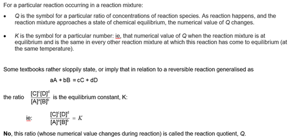
Every function of concentrations becomes constant at equilibrium
Only one function has the same value in all reaction mixtures
Video is in production
Prior familiarity
It would be profitable to have some familiarity with the law of equilibrium (See Module 1103, Equilibrium constants: the law of equilibrium). This module will try to clarify the meaning of this 'law', and to clarify Module 1101 Visualising dynamic chemical equilibrium.
Analogies
Analogies are not the real thing: they have commonalities with the object of interest. We use analogies if those commonalities are useful to understand some conceptual aspect of the real object.
Necessarily, there are also differences – otherwise the analogy would be the real thing. Focus on the commonalities, and not on the differences (unless the differences also helps understanding by contrast).
The setting
In a faraway universe there are two planets – Acidium and Basium.
The Acidians (Let’s denote them by the symbol A) are all identical. And have been since time began. Don’t ask!
And the Basians (B) are all identical, but different from the Acidians.
From some common evolutionary ancestry, they both love to pay hootball.
Whenever the orbits of the two planets are at their closest (every 5021 Earth years) they hold a hootball Interplanetary Cup.
Many games are played. From game to game the numbers of A players, B players and hootballs (symbol H) are different.
The object of the game is simple: Players from the two teams compete for possession of the hootballs. The team in possession of most hootballs after 2 hours is declared the winner.
An overhead drone monitors and analyses the matches, including which players are in possession of a hootball at any moment. On the scoreboard any A player with a hootball is denoted as AH, and any without a hootball is denoted A. Similarly, they keep tabs on the numbers of B (without a hootball) and BH (with a hootball).
At any moment , the number of AH, for example, is recorded as [AH]
Oops they are about to start ……
Game 1 |
Onto the arena go 1000 A players, all with a hootball, and 1000 B players all without a hootball.
So, the starting line-up has [AH] = 1000, [A] = 0, [BH] = 0, [B] = 1000
The game begins. B players attack. You can see some of them wresting hootballs from AHs.
We can represent each such event like this:
So, the starting line-up has [AH] = 1000, [A] = 0, [BH] = 0, [B] = 1000
The game begins. B players attack. You can see some of them wresting hootballs from AHs.
We can represent each such event like this:

After 10 minutes: 130 Bs are in possession of a football. They seem to be pretty competitive! So 130 from the A team are without a football.
[AH] = 870, [A] = 130, [BH] = 130, [B] = 870
After 20 minutes: The B players are in possession of another 70 hootballs – a total of 200.
[AH] = 800, [A] = 200, [BH] = 200, [B] = 800
How long before B team have them all? Let’s keep monitoring ….
After 30 minutes: B team are in possession of 220 hootballs.
[AH] = 780, [A] = 220, [BH] = 220, [B] = 780
The increase is much less than during the previous 10 minutes. Are the B players losing puff?
But wait. The monitor shows us that the apparent slowing down of increase of [BH] is not so much because B players are not winning hootballs as frequently, but because as more and more A players are without hootballs, they are becoming more successful at winning them back.
Oh, A players are winning hootballs from BHs at the same time as B players are winning hootballs from AHs.
After 40 minutes: B team are in possession of 230 hootballs.
[AH] = 770, [A] = 230, [BH] = 230, [B] = 770
After 50 minutes: B team are in possession of 240 hootballs.
[AH] = 760, [A] = 240, [BH] = 240, [B] = 760
After 60 minutes: B team are in still in possession of 240 hootballs.
[AH] = 760, [A] = 240, [BH] = 240, [B] = 760
Final result: The numbers stay the same. They seem to have reached some sort of equilibrium situation. Nothing happening ….. ?
But the monitor shows that transfers of the hootballs are still happening: Players from the A team are wresting hootballs from BHs at the same time as B players are westing footballs from AHs – and at the same rate. Just as many each way in every minute.
Some sort of dynamic equilibrium?
Some sort of dynamic equilibrium?
Game 2
It is obvious from game 1 that A players are more competitive than B players. So the organisers decide to change the starting line-ups: 1000 B players with hootballs and 1000 A players without hootballs.
[AH] = 0, [A] = 1000, [BH] = 1000, [B] = 0
The result: Long before the scheduled end of the game, the match came to dynamic equilibrium: that is, no change in numbers with and without hootballs, but plenty of transfers going on both ways at the same rate.
Final score: [AH] = 760, [A] = 240, [BH] = 240, [B] = 760
So, A players were more successful at winning hootballs from AHs, than the other way around in Game 1. But the final score is the same as in game 1!
Much head-scratching ……. until someone points out ‘Well of course! In both case we had 1000 A players and 1000 B players competing for 1000 hootballs. Same thing!’
Game 3
Since A players are more competitive than the B players, why don’t we use a handicap system and put more B players on the field to see if they can win more than 50% of the hootballs. Let’s allow 2000 B players on the arena.
So, at the start: [AH] = 1000, [A] = 0, [BH] = 0, [B] = 2000
When the match comes to dynamic equilibrium, and there is no point playing any longer, we find that now A players in are in possession of 333 hootballs – more than in game 1, but still not half of the hootballs.
Final score: [AH] = 667, [A] = 333, [BH] = 333, [B] = 1667
Game 4
‘OK’, they say, ‘Let’s give the B team even more advantage. 5000 players’.
So, at the start: [AH] = 1000, [A] = 0, [BH] = 0, [B] = 5000
Will they win all of the hootballs? Well, only 483 - still less than half …..
Final score: [AH] = 517, [A] = 483, [BH] = 483, [B] = 4517
Game 5
Someone points out that another way to even out the competition (other than to increase the number of B players) is to decrease the number of A players.
So 5000 B players (as in Game 4) and only 500 A players with hootballs.
So, at the start: [AH] = 500, [A] = 0, [BH] = 0, [B] = 5000
B players win possession of 304 of the 500 hootballs hootballs.
Final score: [AH] = 196, [A] = 304, [BH] = 304, [B] = 4696
Yes, the B team had won game, but only by having 10 times as many players as the A team.
And when it was all over ...
The Acidians went home in their time machines feeling triumphant, and the Basians went home embarrassed. ‘Exactly the same result as last time 5021 Earth years ago! We’ll show them in the next competition 5021 Earth years from now!’
A nerd is thinking ...
Meanwhile, in the monitoring drone was a nerd. He loved to play with numbers.
He calculated the numerical value of lots of mathematical functions of the final scores. To each different function he assigned an alphabetical letter – going from A to Z.
For example, his sixth randomly chosen function F: F = [BH]/[AH]
Ignoring game 2, because the final numbers were the same as in game 1, he calculated the value of F at the end of each game:
Game 1: F = 240/760 = 0.316
Game 3: F = 333/667 = 0.500
Game 4: F = 483/517 = 0.934
Game 5: F = 304/196 = 1.55
Ah yes, that gives some sense of the final distribution of footballs at equilibrium, taking into account the inherent competitiveness of A players and B players, as well as the relative numbers of each team. Interesting …
He went on calculating the numerical values of randomly decided function. G, H, I, J, K, ………
And then he came to his seventeenth dreamed-up function, Q.
Using this representation of the competition
And then he came to his seventeenth dreamed-up function, Q.
Using this representation of the competition
he thought ‘Well, let’s maybe use the function:
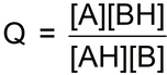
And here is what he calculated for each game at equilibrium:
Within experimental uncertainty, the same value of Q!
To which he had such a reaction that he called this function Q the reaction quotient.
This function has the same numerical value at equilibrium in all arenas! That is not the case for any other function!
So there is a fixed, or constant, value of Q at equilibrium from arena to arena.
They decided to give that particular value of Q the symbol K (In Acidum, the word for constant begins with K.)
Board of IHA (Interplanetary Hootball Association) meeting
A report of the sub-committee for the Interplanetary Cup reads as follows:
This knowledge about the numerical value of Q coming to the same numerical value (call that value K) at equilibrium in every arena allows us to streamline our Interplanetary Cup event.
Because whatever is the value of Q at equilibrium in one game would also be the value of Q in any other game, no matter how many A players, B players, or hootballs.
Once we know the result of one game, we can calculate what the result will be of any other game that we might schedule. It will be the numbers of A, AH, B, and BH at equilibrium that satisfies the condition that Q = K. No point in playing it!
Furthermore, if we know the numbers of A, AH, B, and BH at the start of any game (or even during a game), we can know which team will gain most hootballs before the game comes to equilibrium. It’s like this:
- If at any moment, Q = K, there will be no further net transfers of hootballs. The game is already at equilibrium.
- If Q < K, there will be net transfer such that Q increases (until Q = K). So, there will be an increase of A and BH, and decrease of AH and B: B players will win more hootballs (net) from A players before the situation becomes dynamic equilibrium. This happened in all of the games 1 to 5.
- If Q > K, there will be net transfer such that Q decreases (until Q = K). So, there will be an increase of AH and B and decrease of A and BH: A team players will win more hootballs (net) from B players before the situation becomes dynamic equilibrium.
For example, if we had a situation during a game in which were:
[AH] = 100, [A] = 250, [BH] = 50, [B] = 500
We can calculate that Q = 0.250, which is a larger number than K.
From then until equilibrium is reached, there would be a net increase of B players in possession of hootballs.
IHA Chairman's summing up
Well since all Acidians are identical, and all Basians are identical, and have remained so ever since the Little Bang, we can presume that the results next time willbe the same as they were this time. So there will be no need to transport thousands of players.
We, the Board, will go for a good time …. Delete that, Secretary …… We will go with our computers to calculate the results of the would-be games, and report back on the outcomes of our work.
And what is more, we won’t need to go on the long journey to play the Earthlings, because we can calculate the result in advance.
Uh Oh ... If only he had been talking with Prof Bob
Sorry, Mr. Chairman, but there is a different equilibrium constant K for competitions between different teams.
We won’t be able to calculate the results of Acidium vs. Earth games until they have competed and we have some data to calculate K for those particular reactants .... er, competitors.

Lots of features in common, but not the same.
Finding your way around .....
You can browse or search the Aha! Learning chemistry website in the following ways:
You can browse or search the Aha! Learning chemistry website in the following ways:
- Use the drop-down menus from the buttons at the top of each page to browse the modules chapter-by-chapter.
- Click to go to the TABLE OF CONTENTS (also from the NAVIGATION button) to see all available chapters and modules in numbered sequence.
- Click to go to the ALPHABETICAL INDEX. (also from the NAVIGATION button).
- Enter a word or phrase in the Search box at the top of each page.